Starting with a simple example

Here we consider a simple example of a molecular dynamics simulation for a hydrogen molecule in vacuum. \(H-H\) (a single hydrogen molecule)

Basic knowledge

Let’s go over some basic knowledge before simulations:

• Molecules have an associated energy, which can be divided to potential energy (denoted by \(V\)) and kinetic energy (denoted by \(T\)). Potential energy is related to the coordinates of the atoms in molecules, while kinetic energy is related to the velocity (or momentum) of the atoms.

\begin{aligned} E &= T + V \\ \end{aligned} \begin{aligned} E &= \frac{1}{2} m v^2+V(\vec{q}) \text{ or } E = \frac{p^2}{2m} + V(\vec{q}) \\ \end{aligned}

where \(q\) represents the vector coordinates of atoms and \(p\) represents the momentum of atoms.

• Force is the negative derivative of the energy over coordinates. Since kinetic energy has nothing to do with positions (coordinates), force is also equal to the negative derivative of potential energy over coordinates.

\begin{aligned} F_i &= -\frac{\partial E}{\partial q_i} = - \frac{\partial V}{\partial q_i} \\ \end{aligned}

The construction of theoretical models - generating force fields

Why do we need force fields?

To simulate the motion of hydrogen molecules, we need to know the forces exerted on hydrogen atoms at different positions. These can be used to calculate changes of velocity and coordinates. This is equivalent to knowing the potential energy surface of the \(H_2\) molecule.

How do we get the potential energy surface? The most straightforward way is to calculate the energy by solving Schrödinger equations, and then calculate forces from derivatives. Then our simulation process becomes:

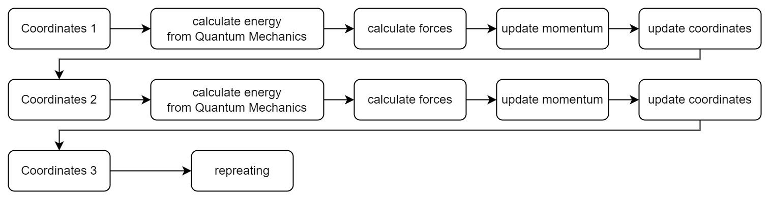
Every time we get a new position in the coordinate space, we need to solve a new set of Schrödinger equations. It is very time-consuming and laborious for complex systems. However, to calculate the motion of hydrogen atoms, we don’t need to know the exact information of the electrons in hydrogen atom, but only the position information of the nucleus. Thus we need the Born-Oppenheimer approximation.

The Born-Oppenheimer approximation is a quantum chemical approximation for electrons. Since nuclei are much heavier than electrons, they move much slower. We can assume that the motion of the nuclei is only affected by the mean-field of electrons.

Simply speaking, we only need to know the positions and forces about the hydrogen nucleus. The influence of electrons can be represented by some force field parameters under approximations. For example, we can approximate the hydrogen molecule as a spring model, and regard the interaction from electrons (or chemical bonds) as a spring. The force generated by the chemical bond is described by the spring coefficient. In this way, we transform the problem of solving Schrödinger equations to calculating the force of a spring:

\begin{aligned} F &= k(x-x_0) \\ \end{aligned}

where \(k\) represents the spring coefficient, and \(x_0\) represents the offset from the equilibrium position. As a result, calculations are greatly simplified. Here, the k (spring coefficient, or force constant) and x0 (equilibrium positions) are simplified force field parameters, also known as the force field.

Note that such simplification can significantly reduce the accuracy of MD simulations, so MD can only reflect the information near equilibrium states. But for macro statistics (e.g. chemical shift, protein contact), it is usually a sufficient description.

The actual force field parameters.

In real MD simulations, almost all inter-atomic and inter-molecular forces are approximated by an analytical expression of classical mechanics. These empirical parameters are obtained by fitting experimental data or data from quantum calculations}(for example, gradient descent optimization. Usually, the format of force fields looks like a combination of terms like:

\begin{aligned} U &=\sum_{\text {bonds }} \frac{1}{2} k_{b}\left(r-r_{0}\right)^{2}+\sum_{\text {angles }} \frac{1}{2} k_{a}\left(\theta-\theta_{0}\right)^{2}+\sum_{\text {torsions }} \frac{V_{n}}{2}[1+\cos (n \phi-\delta)] + \\ \end{aligned} \begin{aligned} \sum_{\text {improper }} V_{i m p}+\sum_{\mathrm{LJ}} 4 \epsilon_{i j}\left(\frac{\sigma_{i j}^{12}}{r_{i j}^{12}}-\frac{\sigma_{i j}^{6}}{r_{i j}^{6}}\right)+\sum_{\text {elec }} \frac{q_{i} q_{j}}{r_{i j}} \\ \end{aligned}

These interactions include:

• Short-range interactions:

  • bonds

  • angles

  • torsion (dihedral angles)

• Long-range interactions

  • Electrostatic interactions (Coulomb interactions, elec)

  • Van der Waals

Preparation for simulation

Now, we have modeled a hydrogen molecule. For simplicity, let the force constant of the hydrogen molecule be \(0.1 kJ/\mathring A^2\). Then let the equilibrium bond length be \(0.5\mathring A\), and the mass of the hydrogen atom is assumed to be (1) (just for demonstration).

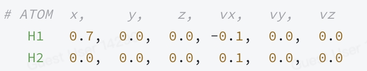
• To start the simulation, we also need the initial conditions (initial conformation and initial velocity). Also for simplicity, we assume that the coordinates of the two atoms are [0.7, 0, 0], [0, 0, 0] (Unit: angstrom), and the velocities are [-0.1, 0, 0], [0.1, 0 , 0] (Unit: angstrom/fs)

  

• Next, let’s set the simulation parameters: since we calculate the differential equation numerically, we need to give the minimum simulation time interval, which is generally set to be 2 fs.(which is actually the grid size for time dimension in finite difference method).

• Set the simulation to 5 steps, so the total simulation time is 10 fs.

• Set the simulated temperature to 300K (this affects the velocity initialization and force field parameters, which should be set before velocity initialization).

Ready? Let’s simulate!

Simulation

(Please be aware that units are omitted for simplicity)

1. Calculate the force on the hydrogen atoms from the initial positions:

\begin{aligned} F_x&=k(x-x_0)=0.1\times(1-0.5)=0.05 \\ \end{aligned}

2. Calculate the accelerations:

\begin{aligned} a_x &= \frac{F}{m}=0.05 \\ \end{aligned}

3. Update velocities:

\begin{aligned} \Delta v_x=a\times \Delta t=0.05 * 2=0.1 \\ \end{aligned} \begin{aligned} \Delta x = v_x \times \Delta t=0.1 * 2=0.2 \\ \end{aligned}

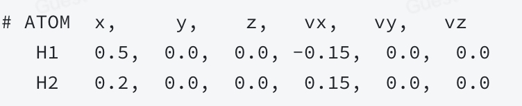
4. Update the coordinates and velocities through the calculation above to obtain new coordinates:

5. (Repeat) Calculate the new force

6. (Repeat) Calculate the new acceleration

Results

Finally, we will obtain positions of H atoms at different times, and these “continuous” motions compose the MD trajectory.

Through long-term MD simulations, we can calculate physical and chemical properties from the trajectories. (such as RMSD changes, conformation transitions, ensemble averaging of physical quantities, etc.)

Notes: Here, the equations from Newtonian mechanics are used for the purposes of demonstration. MD simulation is usually more complicated. Depending on the required ensemble, numerical evolution of partial differential equations will be carried out under specific Hamiltonian mechanics.

We will not introduce the concept of the ensemble in detail here. If you are interested in it, please read the related content about statistical mechanics.